Chapter 5 Case Study: ER Injuries

Exercise 5.8.1

Draw the reactive graph for each app.

Solution.

Solution

Prototype

The prototype application has a single input, input$code, which is used to generate the selected() reactive. This reactive is used directly in 3 outputs, output$diag, output$body_part, and output$location, and it is also used indirectly in the output$age_sex plot via the summary() reactive.

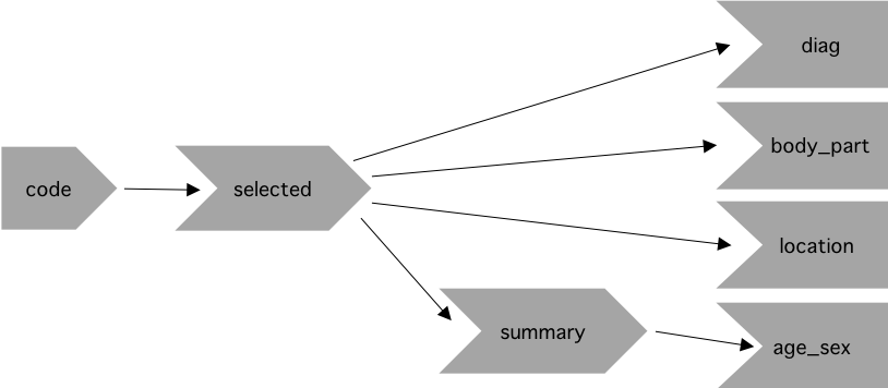
reactive graph - prototype app

Rate vs. Count

Building on the prototype, we create a second input input$y which is used along with the summary() reactive to create the output$age_sex plot.

reactive graph - rate vs. count app

Narrative

Building on the application once more, we create an output$narrative that depends on the selected() reactive and a new input, input$story.

reactive graph - narrative app

Exercise 5.8.2

What happens if you flip fct_infreq() and fct_lump() in the code that reduces the summary tables?

Solution.

Solution

As in the book, we will use the datasets injuries, products, and population appearing here: https://github.com/hadley/mastering-shiny/blob/main/neiss/data.R.

Flipping the order of fct_infreq() and fct_lump() will only change the factor levels order. In particular, the function fct_infreq() orders the factor levels by frequency, and the function fct_lump() also orders the factor levels by frequency but it will only keep the top n factors and label the rest as Other.

Let us look at the top five levels in terms of count within the diag column in the injuries dataset:

injuries %>%
  group_by(diag) %>%
  count() %>%
  arrange(-n) %>%
  head(5)

## # A tibble: 5 × 2
## # Groups:   diag [5]
##   diag                      n
##   <chr>                 <int>
## 1 Other Or Not Stated   44937
## 2 Fracture              43093
## 3 Laceration            39230
## 4 Strain, Sprain        37002
## 5 Contusion Or Abrasion 35259

If we apply fct_infreq() first, then it will reorder the factor levels in descending order as seen in the previous output. If afterwards we apply fct_lump(), then it will lump together everything after the nth most commonly seen level.

diag <- injuries %>%
  mutate(diag = fct_lump(fct_infreq(diag), n = 5)) %>%
  pull(diag)

levels(diag)

## [1] "Other Or Not Stated"   "Fracture"              "Laceration"           
## [4] "Strain, Sprain"        "Contusion Or Abrasion" "Other"

Conversely, if we apply fct_lump() first, then it will label the most frequently seen factor level as “Other”. If afterwards we apply fct_infreq(), then it will label the first level as “Other” and not as “Other Or Not Stated”, which was the case for the previous code.

diag <- injuries %>%
  mutate(diag = fct_infreq(fct_lump(diag, n = 5))) %>%
  pull(diag)

levels(diag)

## [1] "Other"                 "Other Or Not Stated"   "Fracture"             
## [4] "Laceration"            "Strain, Sprain"        "Contusion Or Abrasion"

Exercise 5.8.3

Add an input control that lets the user decide how many rows to show in the summary tables.

Solution.

Solution

Our function count_top is responsible for grouping our variables into a set number of factors, lumping the rest of the values into “Other”. The function has an argument n which is set to 5. By creating a numericInput called rows we can let the user set the number of fct_infreq dynamically. However, because fct_infreq is the number of factors + Other, we need to subtract 1 from what the user selects in order to display the number of rows they input.

library(shiny)
library(forcats)
library(dplyr)
library(ggplot2)

# Note: these exercises use the datasets `injuries`, `products`, and
# `population` as created here:
# https://github.com/hadley/mastering-shiny/blob/main/neiss/data.R

count_top <- function(df, var, n = 5) {
  df %>%
    mutate({{ var }} := fct_lump(fct_infreq({{ var }}), n = n)) %>%
    group_by({{ var }}) %>%
    summarise(n = as.integer(sum(weight)))
}

ui <- fluidPage(
  fluidRow(
    column(8, selectInput("code", "Product",
                          choices = setNames(products$prod_code, products$title),
                          width = "100%")
    ),
    column(2, numericInput("rows", "Number of Rows",
                           min = 1, max = 10, value = 5)),
    column(2, selectInput("y", "Y Axis", c("rate", "count")))
  ),
  fluidRow(
    column(4, tableOutput("diag")),
    column(4, tableOutput("body_part")),
    column(4, tableOutput("location"))
  ),
  fluidRow(
    column(12, plotOutput("age_sex"))
  ),
  fluidRow(
    column(2, actionButton("story", "Tell me a story")),
    column(10, textOutput("narrative"))
  )
)

server <- function(input, output, session) {
  selected <- reactive(injuries %>% filter(prod_code == input$code))
  
  # Find the maximum possible of rows.
  max_no_rows <- reactive(
    max(length(unique(selected()$diag)),
        length(unique(selected()$body_part)),
        length(unique(selected()$location)))
  )
  
  # Update the maximum value for the numericInput based on max_no_rows().
  observeEvent(input$code, {
    updateNumericInput(session, "rows", max = max_no_rows())
  })
  
  table_rows <- reactive(input$rows - 1)
  
  output$diag <- renderTable(
    count_top(selected(), diag, n = table_rows()), width = "100%")
  
  output$body_part <- renderTable(
    count_top(selected(), body_part, n = table_rows()), width = "100%")
  
  output$location <- renderTable(
    count_top(selected(), location, n = table_rows()), width = "100%")
  
  summary <- reactive({
    selected() %>%
      count(age, sex, wt = weight) %>%
      left_join(population, by = c("age", "sex")) %>%
      mutate(rate = n / population * 1e4)
  })
  
  output$age_sex <- renderPlot({
    if (input$y == "count") {
      summary() %>%
        ggplot(aes(age, n, colour = sex)) +
        geom_line() +
        labs(y = "Estimated number of injuries") +
        theme_grey(15)
    } else {
      summary() %>%
        ggplot(aes(age, rate, colour = sex)) +
        geom_line(na.rm = TRUE) +
        labs(y = "Injuries per 10,000 people") +
        theme_grey(15)
    }
  })
  
  output$narrative <- renderText({
    input$story
    selected() %>% pull(narrative) %>% sample(1)
  })
}

shinyApp(ui, server)

Exercise 5.8.4

Provide a way to step through every narrative systematically with forward and backward buttons.

Advanced: Make the list of narratives “circular” so that advancing forward from the last narrative takes you to the first.

Solution.

Solution

We can add two action buttons prev_story and next_story to iterate through the narrative. We can leverage the fact that whenever you click an action button in Shiny, the button stores how many times that button has been clicked. To caculate the index of the current story, we can subtract the stored count of the next_story button from the previous_story button. Then, by using the modulus operator, we can increase the current position in the narrative while never go beyond the interval [1, length of the narrative].

library(shiny)
library(forcats)
library(dplyr)
library(ggplot2)

# Note: these exercises use the datasets `injuries`, `products`, and
# `population` as created here:
# https://github.com/hadley/mastering-shiny/blob/main/neiss/data.R

count_top <- function(df, var, n = 5) {
  df %>%
    mutate({{ var }} := fct_lump(fct_infreq({{ var }}), n = n)) %>%
    group_by({{ var }}) %>%
    summarise(n = as.integer(sum(weight)))
}

ui <- fluidPage(
  fluidRow(
    column(8, selectInput("code", "Product",
                          choices = setNames(products$prod_code, products$title),
                          width = "100%")
    ),
    column(2, numericInput("rows", "Number of Rows",
                           min = 1, max = 10, value = 5)),
    column(2, selectInput("y", "Y Axis", c("rate", "count")))
  ),
  fluidRow(
    column(4, tableOutput("diag")),
    column(4, tableOutput("body_part")),
    column(4, tableOutput("location"))
  ),
  fluidRow(
    column(12, plotOutput("age_sex"))
  ),
  fluidRow(
    column(2, actionButton("prev_story", "Previous story")),
    column(2, actionButton("next_story", "Next story")),
    column(8, textOutput("narrative"))
  )
)

server <- function(input, output, session) {
  selected <- reactive(injuries %>% filter(prod_code == input$code))
  
  # Find the maximum possible of rows.
  max_no_rows <- reactive(
    max(length(unique(selected()$diag)),
        length(unique(selected()$body_part)),
        length(unique(selected()$location)))
  )
  
  # Update the maximum value for the numericInput based on max_no_rows().
  observeEvent(input$code, {
    updateNumericInput(session, "rows", max = max_no_rows())
  })
  
  table_rows <- reactive(input$rows - 1)
  
  output$diag <- renderTable(
    count_top(selected(), diag, n = table_rows()), width = "100%")
  
  output$body_part <- renderTable(
    count_top(selected(), body_part, n = table_rows()), width = "100%")
  
  output$location <- renderTable(
    count_top(selected(), location, n = table_rows()), width = "100%")
  
  summary <- reactive({
    selected() %>%
      count(age, sex, wt = weight) %>%
      left_join(population, by = c("age", "sex")) %>%
      mutate(rate = n / population * 1e4)
  })
  
  output$age_sex <- renderPlot({
    if (input$y == "count") {
      summary() %>%
        ggplot(aes(age, n, colour = sex)) +
        geom_line() +
        labs(y = "Estimated number of injuries") +
        theme_grey(15)
    } else {
      summary() %>%
        ggplot(aes(age, rate, colour = sex)) +
        geom_line(na.rm = TRUE) +
        labs(y = "Injuries per 10,000 people") +
        theme_grey(15)
    }
  })
  
  # Store the maximum posible number of stories.
  max_no_stories <- reactive(length(selected()$narrative))
  
  # Reactive used to save the current position in the narrative list.
  story <- reactiveVal(1)
  
  # Reset the story counter if the user changes the product code. 
  observeEvent(input$code, {
    story(1)
  })
  
  # When the user clicks "Next story", increase the current position in the
  # narrative but never go beyond the interval [1, length of the narrative].
  # Note that the mod function (%%) is keeping `current`` within this interval.
  observeEvent(input$next_story, {
    story((story() %% max_no_stories()) + 1)
  })
  
  # When the user clicks "Previous story" decrease the current position in the
  # narrative. Note that we also take advantage of the mod function.
  observeEvent(input$prev_story, {
    story(((story() - 2) %% max_no_stories()) + 1)
  })
  
  output$narrative <- renderText({
    selected()$narrative[story()]
  })
}

shinyApp(ui, server)